Simulate a dataset for the Function Linear Regression model.
sim(param, verbose = FALSE)Arguments
- param
a list containing:
- beta_shapes
a character vector. The qth item indicates the shape of the coefficient function associated to the qth functional covariate.
- beta_functions
a list containing numerical vectors to define the beta functions
- n
an integer, the sample size.
- p
a vector of integers, the qth component is the number of times for the qth covariate.
- Q
an integer, the number of functional covariates.
- autocorr_diag
a list of numerical vectors (optional), the qth vector is the diagonal of the autocorrelation matrix of the qth functional covariate.
- autocorr_spread
a vector of numerical values (optional) which are related to the autocorrelation of the functional covariates.
- grids
a list of numerical vectors (optional), the qth vector is the grid of time points for the qth functional covariate.
- grids_lim
a list of numerical vectors (optional), the qth item is the lower and upper boundaries of the domain for the qth functional covariate.
- link
a function (optional) to simulate data from the Generalized Functional Linear Regression model.
- mu
a numerical value (optional), the 'true' intercept of the model.
- r
a nonnegative value (optional), the signal to noise ratio.
- x_shapes
a character vector (optional). The qth item indicates the shape of the functional covariate observations.
- verbose
write stuff if TRUE.
Value
a list containing:
- Q
an integer, the number of functional covariates.
- y
a numerical vector, the outcome observations.
- x
a list of matrices, the qth matrix contains the observations of the qth functional covariate at time points given by
grids.- grids
a list of numerical vectors, the qth vector is the grid of time points for the qth functional covariate.
- betas
a list of numerical vectors, the qth vector is the 'true' coefficient function associated to the qth covariate on a grid of time points given with
grids.
Examples
library(RColorBrewer)
param <- list(Q=2,n=25,p=c(50,50),grids_lim=list(c(0,1),c(-1,2)))
data <- sim(param)
data$y
#>  [1] -2.82937439  2.80104399  2.97512240  7.65717553  1.47814297 -0.71020040
#>  [7]  1.35608417  2.82028131  3.22951886  1.80464865  2.36689602  1.55424369
#> [13] -2.58164496  3.22195689  1.88025746 -1.01501727  0.03884157 -3.20717225
#> [19]  0.33475070 -4.43567693  2.67571759  3.36010023  3.36686298 -0.91862471
#> [25]  3.04193065
cols <- colorRampPalette(brewer.pal(9,"YlOrRd"))(10)
q=2
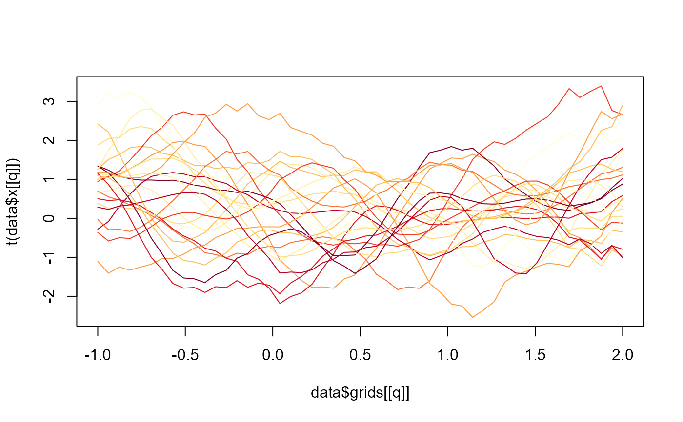
matplot(data$grids[[q]],t(data$x[[q]]),type="l",lty=1,col=cols)

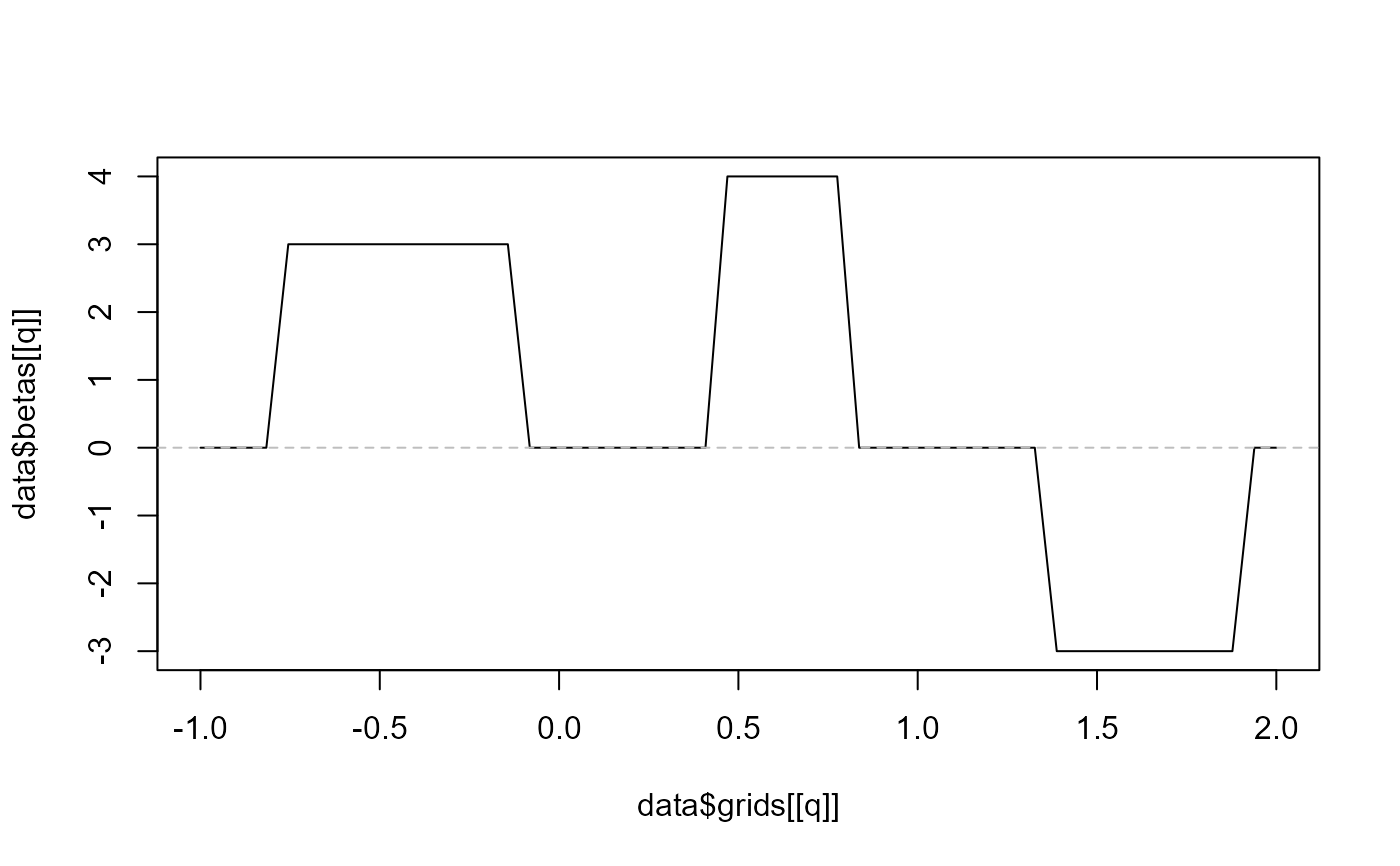
plot(data$grids[[q]],data$betas[[q]],type="l")
abline(h=0,lty=2,col="gray")
