Simulate functional covariate observations.
sim_x(param)Arguments
- param
a list containing :
- grid
a numerical vector, the observation times.
- n
an integer, the sample size.
- p
an integer, the number of observation times.
- diagVar
a numerical vector (optional), the diagonal of the autocorrelation matrix.
- dim
a numerical value (optional), the dimension of the Fourier basis, if "shape" is "Fourier" or "Fourier2".
- ksi
a numerical value (optional) related to the observations correlation.
- x_shape
a character vector (optional), the shape of the observations.
Value
a matrix which contains the functional covariate observations at time
points given by grid.
Details
Several shape are available for the observations: "Fourier", "Fourier2", "random_walk", "random_sharp", "uniform", "gaussian", "mvgauss", "mvgauss_different_scale", "mvgauss_different_scale2", "mvgauss_different_scale3" and "mvgauss_different_scale4".
Examples
library(RColorBrewer)
### uniform
param <- list(n=15,p=100,grid=seq(0,1,length=100),x_type="uniform")
x <- sim_x(param)
cols <- colorRampPalette(brewer.pal(9,"YlOrRd"))(15)
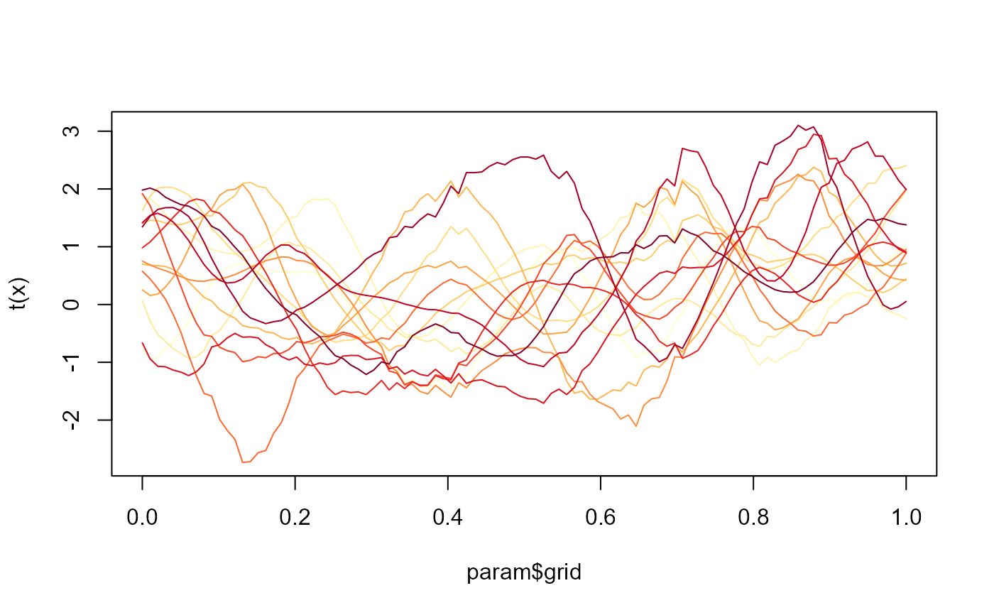
matplot(param$grid,t(x),type="l",lty=1,col=cols)
